Introduction to Text Data Preprocessing

Introduction

Overview

I became interested in Natural Language Processing (NLP) because of the Coursera Data Science Specialization Capstone Project, where NLP was used to process a large corpus dataset to build a word prediction app.

After the project, I wanted to document my (extremely) basic understanding of NLP and further perfect my prediction model (as always ;)), hence this NLP word prediction series. The series covers the following:

1. Preprocessing
2. Exploratory data analysis
3. Model building
4. Prediction

The blog series is meant to be more explanatory and fewer codes. All the codes can be found separately in my word-prediction Github page. You can also find the original Capstone Project documentation in my Capstone Project Github page.

This is the first part of the NLP word prediction series, text preprocessing.

Basics

Corpus

A corpus (plural corpora) is a large collection of structured text data, it may contain a single language or multiple languages

The basic steps of text data processing include:

1. Tokenization
2. Word filtering
3. Normalization
4. Noise removal

We will use the quanteda package for R and the Capstone Project data for the word prediction project.

Setup

1. Packages

suppressMessages(library(quanteda))
suppressMessages(library(readtext))
suppressMessages(library(stringi))
suppressMessages(library(kableExtra))
suppressMessages(library(ggplot2))
suppressMessages(library(cowplot))
suppressMessages(library(reshape2))

2. Read in data

data_blog <- texts(readtext(file = paste0(dataDir, "/en_Us.blogs.txt")))
data_news <- texts(readtext(file = paste0(dataDir, "/en_US.news.txt")))
data_twt <- texts(readtext(file = paste0(dataDir, "/en_US.twitter.txt")))

The readtext() function loads the text files into a data.frame object. The text can be accessed with the text() method. To prevent all the texts from printing (don’t use head()), we can use the stri_sub() function to print out the desired characters (1st to 80th) of the texts of the data_ objects.

stri_sub(data_blog, 1, 80)

[1] “In the years thereafter, most of the Oil fields and platforms were named after p”

3. Basic summary

data_sum <- data.frame("Source" = c("Blog", "News", "Twitter"),
                       "Lines" = c(stri_count_fixed(data_blog, "\n"),
                                   stri_count_fixed(data_news, "\n"),
                                   stri_count_fixed(data_twt, "\n")))

Source	Lines
Blog	899287
News	1010241
Twitter	2360147

We can count the lines by counting the newline characters \n in the text

Preprocessing

1. Combining corpera

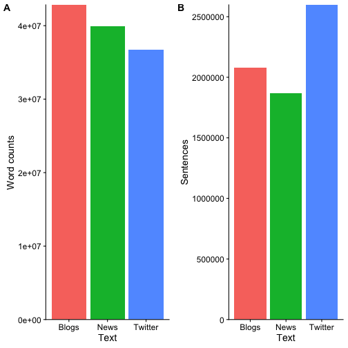
Since we actually have corpus data from three sources, blogs, news, and Twitter, we can first construct individual corpus from each data source and combine all data into a corp_all variable that is still a corpus object. The summary information can be calculated from the combined corpus and plot the distribution of words and sentences based on the different data sources

corp_blog <- corpus(data_blog)
corp_news <- corpus(data_news)
corp_twt <- corpus(data_twt)
corp_all <- corp_blog + corp_news + corp_twt
corp_sum <- summary(corp_all)

Text	Types	Tokens	Sentences
en_US.blogs.txt	482434	42840147	2077533
en_US.news.txt	431664	39918314	1868674
en_US.twitter.txt	566950	36719645	2598128

Prior to any preprocessing, it seems like blogs contain the most words and Twitter the most sentences

2. Tokenization

Tokenization refers to the process of separating (segmenting) a large paragraph into words, phrases, sentences, symbols, or other elements called tokens. Tokenization allows the identification of basic units for downstream text analysis. Usually, during tokenization, characters like punctuations and numbers are discarded. However, what to discard is mainly dependent on the goal of the downstream analysis

We first want to tokenize the words with the tokens() function, which splits the text into individual words. For downstream analysis, numbers, punctuations, symbols, Twitter characters, and urls are removed since they are likely not useful to the next word prediction.

tok <- tokens(corp_all, what = "word",
              remove_numbers = TRUE, remove_punct = TRUE,
              remove_symbols = TRUE, remove_twitter = TRUE,
              remove_url = TRUE)
tok_sum <- summary(tok)

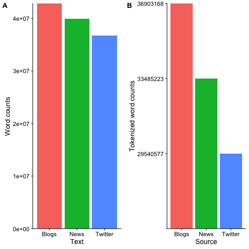
Similarly, we can look at the distribution of tokenized words from each data source

	Length	Class	Mode
en_US.blogs.txt	36903168	-none-	character
en_US.news.txt	33485223	-none-	character
en_US.twitter.txt	29540577	-none-	character

We can now compare the differences in words from all sources before and after tokenization

3. Profanity filtering

Word filtering, as suggested by its name, is the process to filter out unwanted words. This is usually an optional step that depends on the downstream application

The next step is to remove any profanity since we wouldn’t want a word prediction app to suggest bad words

if (!file.exists(paste0(dataDir, '/badWords.txt'))) {
  download.file('https://raw.githubusercontent.com/shutterstock/List-of-Dirty-Naughty-Obscene-and-Otherwise-Bad-Words/master/en',
                dest = paste0(dataDir, '/badWords.txt'),
                method = 'curl', quiet = T)
  }
prof <- readLines(paste0(dataDir, '/badWords.txt'), skipNul = T)

The list of profanity is obtained from here.

tok <- tokens_remove(tok, pattern = prof)

We will directly overwrite the tokenized tok variable

4. Normalization

Normalization is the process to reduce inflected and derived words to their “roots”, with the hopes of making all the words “equal”. This includes converting texts to the same case (upper or lower) and making the text into a single canonical form. For instance, type, typed, typing, and typed are all the same words, and would be reduced to “type” during the normalization process. The two types of normalization are as follows

Stemming

Word stemming is a brute force way to normalize words by chopping the end off directly, hoping that words will be normalized correctly most of the time. For example, argue, argues, argued, arguing, will all be reduced to the stem argu. As shown here, the stem doesn’t have to be an actual word but should represent a way to summarize the same word with different forms.

Lemmatization

Lemmatization refers to a more careful normalization by analyzing the vocabulary and morphology to remove the inflectional endings and only return the correct root or the dictionary form of the word. In the example above, argue will be returned.

Since lemmatization is slightly more complicated and computationally expensive, we will use stemming to normalize the tokens. We can perform stemming with the dfm() function that constructs a document-feature matrix to summarize the tokens

dfm1 <- dfm(tok, tolower = TRUE, stem = TRUE)

5. Remove stop words

Stop words refer to the most common words in a language that is not always valuable for analysis and doesn’t change the overall tone of the sentence (to, and, for, from, this, that, etc.). Removal of stop words often depends on the application.

In our case, we would want to include stop words for modeling and prediction. But to explore word frequencies, we will (temporarily) remove the stop words.

dfm1_rm <- dfm(dfm1, tolower = TRUE, remove = stopwords("english"))

Conclusion

I hope this is an informative post to introduce the basics of text data preprocessing using the quanteda package. Usually, data preprocessing is the boring (but essential) part, but I actually have a lot of fun learning about textual data processing. Now that we have cleaned up our corpora, the next step is to do some interesting exploratory data analysis!

References

1. quanteda
2. Basics of NLP